Contents
Trend curve
The actions to be taken will be controlled through measurements of variables that have a trend curve over time, for example:
- pressure;
- temperature;
- flow;
- level;
- vibration;
- moisture;
- dielectric strength;
- dimensions;
- PH;
- chemical elements.
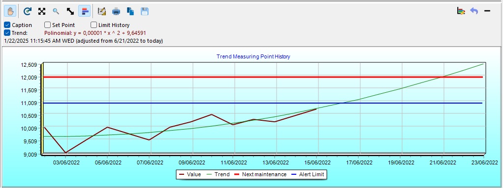
In trend scheduling, when reaching an established maximum or minimum value, Engeman® will indicate the need for maintenance through work orders, alarms, or issuance. The user can set alarm levels as much as necessary.
Data measurement, also known as collection, can be performed through manual notes and through equipment intended for this purpose, such as sensors and PLC computers. This measurement and data collection equipment may be linked directly to the asset point of maintenance or maybe portable for use at various points, such as thermal imaging cameras, for instance.
The information obtained over time creates a trend curve of the measured variable. This trend curve will be calculated by mathematical regressions defined by the user or automatically by Engeman®.
Regressions can be linear, logarithmic, exponential, potentiation, or polynomial. This curve will establish a mathematical function of values vs. date, thus making it possible to determine the future maintenance date from the date on which the last maintenance of the asset was performed.
If you request calculations for a longer period, Engeman® calculates the maintenance dates within the period, based on the mathematical function generated by the measurements of the first maintenance.
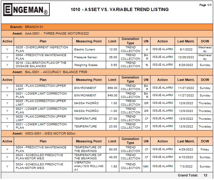
Necessary precautions for trend scheduling process
- If the measurements do not display a trend, expressed by a mathematical function over time, this process should not be used. In this case, it will be recommended to use periodic or event-based scheduling;
- Measurements must be made systematically, which will require greater demand for resources and control of actions. You can create plans with periodic scheduling to control this process, for example;
- In the case of automatic measurements, verify data collection reliability and predict contingencies;
- Rationalizes the process of measuring points number;
- Use Engeman® Mobile for the manual data collection process.
In addition to issuing work orders and proximity alarms on scheduled dates, Engeman® allows you to view measurements and future maintenance dates:
- Through measurements and typing of the numbers, Engeman® will start alarms or calculate the performing W.O. date, when there is a tendency for the variables to exceed the established limits.
- The W.O. closing automatically reschedules the next performing date, with no need to perform a new startup.
In the same way as periodic scheduling, Engeman® issues consecutive W.O.s if the period requested by the user is long enough to allow the process. In this way, the first calculated W.O. will be based on real measurements, and the others will be calculated through the mathematical function established by the first W.O.
How do you create a trend scheduling at Engeman®?
The correct measuring point definition is of utmost importance for trend scheduling, as it will determine the startup of the analysis.
Let’s see what information is needed in Engeman® to define them well:

- Measuring Point Description
-
- Maximum collections: maximum number of collections that will be used for the regression calculation. This field can be left blank so that the entire history is checked in the regression calculation. If informed, only the last numbers will be analyzed to calculate the trend of production evolution.
- History Period: such as the previous item, the historical period is also optional information. Determines the period of days that will be used, from the last collection to the first, in the curve evolution trend calculation.
- Measuring Unit
-
- Number of decimal places: Specifies the number of decimal places used for the data collected. Leave this field blank so that there is no formatting.
- Measuring Point Type
Filling in is mandatory. It defines better organization for the asset measuring points register, makes the routine of moving assets more dynamic, provides less work to the user, and restricts possible duplications of Measuring Point Types of assets.
ATTENTION: this field is the only information that guarantees the differentiation between the measuring points of the same asset. Therefore, if there are several measuring points of the same type in the same asset, a different type must be registered for each of them.
- Set point: Indicates the normal number of the measured variable.
- Regression type: Determines the regression type to be used for trend graphs and W.O. generation. There are five regression types: Linear, Logarithmic, Power, Exponential, and Polynomial, in addition to the Automatic type (suggested default), where the best curve is automatically determined according to the data.
Let’s see more information about regression curves.
Regression Curves or Trend Lines
Trend lines are used to graphically display data trends and to analyze problems related to projections. This type of analysis is also called regression analysis (regression analysis: a form of statistical analysis used to make predictions). Regression analysis calculates the relationship between variables so that a given variable can be predicted from one or more different variables).
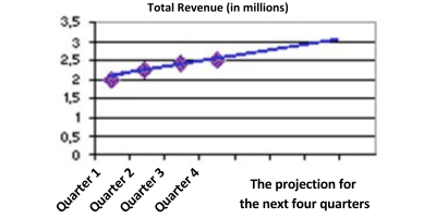
Using regression analysis, you can project a trend line on a graph in addition to the actual data to predict future data. For example, the following chart uses a linear trend line with a projection four months in advance to display the trend for revenue growth.
Types of Trend Lines
See below the types of trend lines we have:
-
Linear
The linear trend line is the straight line that best suits and is used in simple sets of linear data. Your data is linear if the pattern of the data points resembles a line. The linear trend line usually shows that something is increasing or decreasing by a constant percentage.
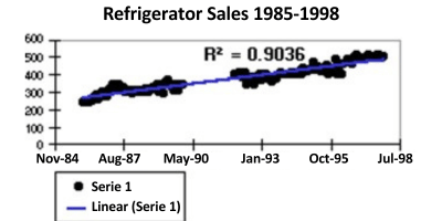
In the following example, a linear trend line displays that refrigerator sales have had steady growth over 13 years. Note that the value of R squared is 0.9036, which corresponds to a good fit of the row to data.
-
Logarithmic
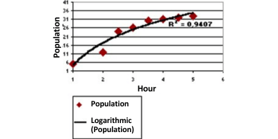
The logarithmic trend line is a fitted curved line used when the percentage of change in the data increases and decreases rapidly and then stabilizes. A logarithmic trend line can use negative and/or positive values.
The following example uses a logarithmic trend line to illustrate the predicted growth of the animal population in a defined area, displaying that while the population has stabilized, the space available for animals has decreased. Note that the value of R squared is 0.9407, which corresponds to a good fit of the row to the data.
-
Polynomial
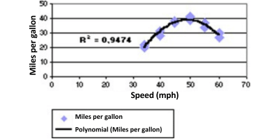
The polynomial trend line is a curved line used when there is data fluctuation. It is useful, for example, to analyze the gains and losses of a set of data. The order of the polynomial can be determined by the number of data fluctuations or by the number of oscillations (maxima and minimum) of the curve. Usually, a polynomial trend line number 2 has only a high or low. As a rule, number 3 has two highs or lows. Number 4 has more than three.
The following example shows a polynomial trend line number 2 (a maximum) to illustrate the relationship between speed and fuel consumption. Note that the value of R squared is 0.9474, which corresponds to a good fit of the line to the data.
-
Power
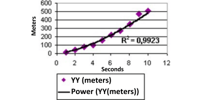
A power trend line is a curved line used with data sets that compare measurements that increase at a specific rate – for example, the acceleration of a race car at one-second intervals. You cannot create a power trend line if the data has 0 or negative numbers.
In the following example, the acceleration data is displayed by the distances in meters per second. The power trend line displays the acceleration increase. Note that the number of R squared is 0.9923, which corresponds to an almost perfect fit of the line to the data.
-
Exponential
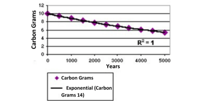
The exponential trend line is a curved line, used when data numbers increase or decrease by higher and higher percentages. You can’t create an exponential trend line if the data includes zero or negative numbers.
In the following example, the exponential trend line is used to illustrate the decrease in carbon-14 content as an object ages. Note that the number of R squared is 1, which means that the line fits the data perfectly.
Important: In most cases, in Engeman®, using the automatic option based on the collection history of the measuring point, will define the best function to be used. However, if a certain measuring point has the characteristic of oscillating too much, suggesting a frequency graph, choose to use linear regression, which will be less sensitive to momentary variations.
Conclusion
Trend scheduling is perhaps the most complex for managing a maintenance area, but even so, the benefits of predictive maintenance are clear.
When predictive maintenance effectively functions as a maintenance strategy, maintenance is only performed when it is needed, just before the likely failure occurs. This brings cost reduction, with:
- minimization of equipment maintenance time;
- minimization of production hours lost to maintenance;
- minimizing the cost of spare parts and supplies.
Applying predictive maintenance can lead to an ROI increase of approximately:
- 25%-30% reduction in maintenance costs;
- 70%-75% reduction in breakdowns;
- 35%-45% reduction in downtime.
These cost savings do, however, come at a price. Some condition monitoring techniques are expensive and require specialized and experienced workers, along with the integration of these techniques with Engeman®, for data analysis to be effective.
However, despite the high initial cost, it allows maintenance to be performed only when necessary, helping facilities cut costs, save time, and maximize resources.
In the next article, we will continue in the world of maintenance by asset conditions, but we will be talking about a scenario that few still use, but which also offers a lot for management: By Event Schedules.
See you there!
Also, follow the first articles of the Maintenance Schedule series at Engeman®:
- 1st – Periodic – Time-Based Maintenance (TBM)
- 2nd – Specific Date – Time-Based Maintenance (TBM)
- 3rd – Cumulative – Condition-Based Maintenance (CBM)


